What I Built
I am a big geek about information retrieval and I’ve been eagerly awaiting this lesson. I finally get to build the thing! I built a very simple app with Claude and ChromaDB: A PM Knowledge Assistant and Strategy Advisor that provides grounded responses based on my documents.
Oh, and I also made my first golden set to define baseline metrics for my Feature Spec Generator.
Embeddings
The first step was to turn meaning into math. Wait. Sigh.
No, apparently the first step is to solve this Python 3.14 + ChromaDB (ChromaDB’s Pydantic v1, to be precise) incompatibility. Had to create another environment, venv-rag, with Python 3.12. Caught Claude throwing shade at me while it was thinking. “He’s not super CLI-savvy…”
Ok, NOW it was time to turn meaning into math. embeddings_intro.py was my first embedding script, using OpenAI’s text-embedding-3-small to get embedding vectors for selected text inputs and measure their similarity:
- text_a = “How do I configure Adobe Target for A/B testing?”
- text_b = “Setting up experiments in our personalization platform”
- text_c = “What’s our Q3 revenue forecast?”
The cosine similarity results for A vs B were nearly 3x higher than A vs C:
- A vs B: 0.4120 (similar topics)
- A vs C: 0.1437 (different topics)
- Difference: 0.2684
The system made a semantic match with zero keyword overlap. My library science colleagues would salivate if they saw this.
Vector Store
Oh, crap. Another database technology. Here we go. Vectors, chunks, embeddings. It was a lot to digest (ingest?). Yet somehow intuitive.
Today’s build was a document ingestion pipeline (rag_pipeline.py) with ChromaDB that performed the following operations:
- Connects to a local ChromaDB instance and creates (or opens) a persistent collection
- Reads source documents (in this case, a 5 long text snippets about B2B personalization)
- Splits each document into chunks with configurable size and overlap
- Generates embeddings for each chunk using OpenAI’s
text-embedding-3-smallmodel - Upserts the embedded chunks into ChromaDB with metadata (source filename, chunk index)
- Accepts a natural language query, embeds it, and runs a similarity search against collection
- Returns the top-K matching chunks ranked by cosine distance score
Two things I looked for: does each query find the right documents, and do the distance scores make sense (lower = more relevant)? The answer to both: yes. So far, so good.
Then I tried searched for something (Salesforce integration) that was NOT in the documents. ChromaDB still returned its best-match chunks. The distance scores were higher, but it still returned chunks. It doesn’t have a “no match found” threshold built in. However, Claude looked at the retrieved chunks, recognized none of them were about Salesforce, and said it didn’t have that information instead of making something up. A grounded answer. Yay!
BUT … that’s only because my Python script explicitly instructed Claude to only answer from the provided context.
Answer questions based ONLY on the provided context documents.
2. If the context doesn't contain enough information to answer, say so clearly.
3. Always cite which source document(s) you drew from.
4. Never make up information that isn't in the context.
5. If asked something outside the provided context, acknowledge this and offer
   to help with what you do have context for.
Without that system prompt guardrail, Claude would have happily invented an answer to my Salesforce question.
RAG Pipeline
Yesterday showed me how retrieval works and that my guardrails kept Claude from hallucinating. Today was the day the whole week clicked. I connected ChromaDB retrieval to Claude generation and built the full RAG retrieve → generate pipeline in rag_assistant.py.
This time, I ingested five synthetic (AI-generated) documents to simulate the following:
- Account-based marketing strategy
- Personalization platform details
- Data signal definition framework
- Quarterly performance metrics
- A personalization roadmap
These are the kinds of documents a PM might need to sift through page by page for hours on end with the midnight oil burning.
The architecture was straightforward: embed the question, pull the top 3 chunks from ChromaDB, inject them as context, let Claude generate. Same five grounding rules from Day 2, same belt-and-suspenders constraint in the user prompt. Then I ran four tests to answer the question of the week: does RAG actually improve output quality?
Grounding Test
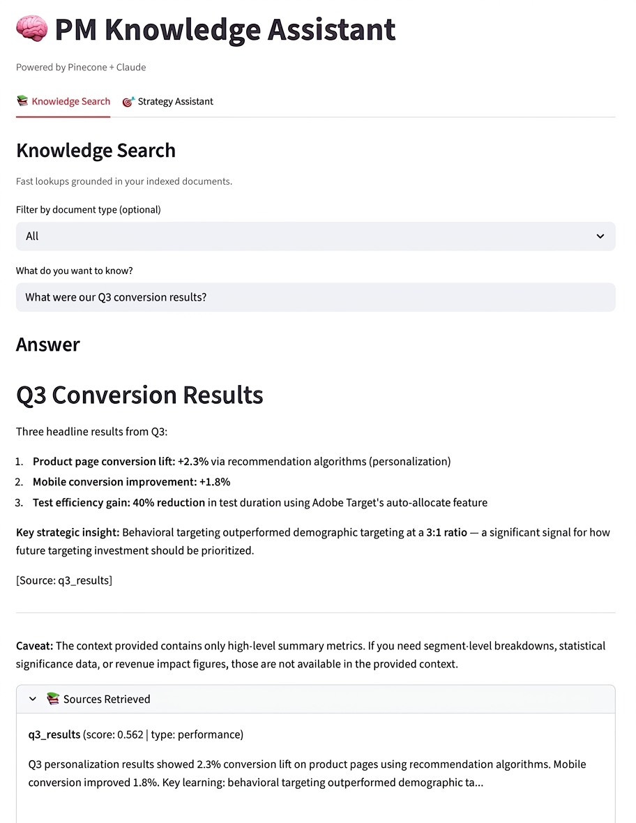
I asked “What was our conversion lift from personalization?” twice: once with the RAG pipeline, once with the same model and prompt but no retrieved context. With RAG, Claude cited the specific 2.3% from our Q3 data. Without RAG, it gave me generic industry benchmarks about personalization typically driving 5-15% lift. Same model. Same prompt. Completely different answers. One is useful to my team. The other is a Google search.
Cross-Document Synthesis Test
I asked “what’s working in our personalization program?”… Claude pulled from both the quarterly metric and the signal definitions, connected the behavioral targeting 3:1 ratio to the signal-first architecture in our scoring framework, and drew a novel insight: “the behavioral signal-first approach is validated by the data.” I didn’t tell it to connect those documents. The retrieval surfaced relevant chunks from both, and Claude reasoned across the evidence on its own.
Out-of-Context Behavior
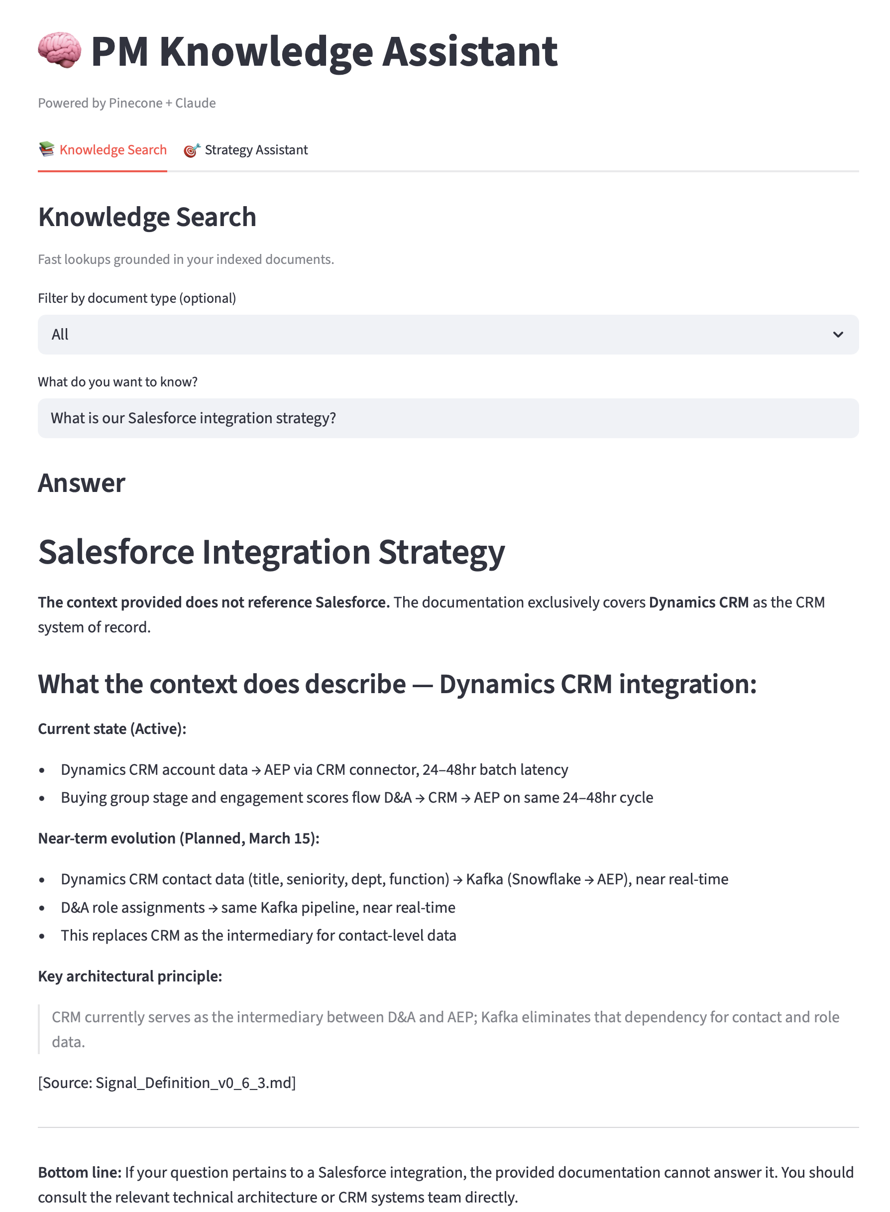
I asked about our Salesforce integration strategy, which isn’t in any of the documents I ingested. ChromaDB still returned its top 3 chunks (it always does; there’s no “no match found” threshold). But Claude read the retrieved chunks, recognized none of them were about Salesforce, and said it didn’t have that information. Then it listed what it did have context for. No hallucination. No confident-sounding nonsense borrowed from training data.
RAG Quality Deep Dive
Thursday was a full deep dive into three retrieval quality techniques: hybrid search, re-ranking, and metadata filtering. The pipeline works. The grounding test proved it. But “it finds the right documents” is a low bar. The goal for today was to see if I could make retrieval “smarter”: returning better chunks, filtering out noise, and handling queries where the top results by distance score aren’t actually the most relevant.
Hybrid Search
This one was a letdown. It was supposed to combine semantic search (meaning) with keyword search (exact terms) for better recall. But keyword matching never fired. ChromaDB’s $contains filter is case-sensitive and only matches exact substrings. Semantic search still found the right docs, just without the boost layer. Claude explained later Chrome DB is not good at this. A real implementation needs a dedicated keyword engine like Elasticsearch alongside the vector store. Which is obviously overkill for a five-document collection.
Re-Ranking (With Claude Haiku)
This one quietly did real work. The idea: after ChromaDB returns the top chunks by distance score, send them to Claude Haiku for a second pass. Haiku reads each chunk and scores its actual relevance to the query, not just its vector proximity. This technique caught things that distance scores alone couldn’t. Claude correctly pruned irrelevant chunks. It dropped Adobe Target config from a user persona query, but kept it for an integration query. Same chunk, different queries, correct judgment both times. This seems like the technique that would matter most at scale with hundreds of documents that contain a mix of relevance and noise.
Metadata filtering
This technique is a no-brainer. Each chunk carries metadata tags from ingestion (source file, category). Filtering by category before the similarity search narrows the result set to the right domain. I tested with a performance-related query: the performance filter returned Q3 results at distance 0.662, while the technical filter returned signal definitions at 0.590. The distance scores alone would have preferred the wrong document. The filter fixed it. This maps directly to my real work: strategy docs shouldn’t surface for technical queries and vice versa.
Day 5: Knowledge Assistant Deployed
Four days of building pipelines in Python scripts. Time to put it in front of people.
I converted rag_assistant.py into a Streamlit app, reusing the patterns from the Week 5 Feature Spec Generator deployment: session state for multi-step flow, secrets management for API keys, spinners for the long embedding and generation calls. The conversion was straightforward because the RAG pipeline has a clean two-step architecture (retrieve, then generate) that maps naturally to Streamlit’s rerun model.
The app added a few things the CLI script didn’t have. A file upload widget lets users ingest their own documents into the vector store without touching the command line. Source citations display below each answer so the user can see which chunks Claude drew from and verify the grounding. The vector store persists across sessions, so documents ingested once stay available.
Deployment to Streamlit Cloud followed the same workflow as Week 5: push to a dedicated GitHub repo, connect in the Streamlit Cloud dashboard, configure secrets, deploy. Ta-da!
Two deployed tools now live: Feature Spec Generator and Knowledge Assistant. The first is a single-agent prompt wrapper. The second has an entire retrieval pipeline underneath it. From the user’s perspective, both are just a text box and a response. The complexity is invisible, which is exactly where it should be.
Day 6: Evaluation Foundations
Bonus day! Now that I have real users for my Feature Spec Generator, I’m getting questions about consistency and quality, and I need to know: “Is my AI product actually good?”
Claude presented me with an “extra credit” assignment to build a golden set of 10 test cases for my Feature Spec Generator. I built evaluation.py with 5 test cases and two evaluation layers:
- A set of rule-based checks (are the required sections present? is the output long enough?)
- An LLM-as-judge scorer that rates overall quality on a 5-point scale
The results from the first run were weird. The rule-based checks passed at 94%, which seemed right. But the LLM judge scored 4.2/5.0, docking points for missing acceptance criteria and incomplete technical requirements.
I looked at the specs. The acceptance criteria were there. So were the technical requirements. Then I discovered a truncation bug: the judge was evaluating only the first 3,000 chars and docking points for sections it couldn’t see. So I bumped the limit to 6,000 characters and ran it again. 94% rule-based, 4.6/5.0 LLM judge. Baseline recorded.
What I Learned
Embeddings Are Inexpensive
AI economics have become a much more central topic than I anticipated at the outset of this learning path. What I learned this week is that embeddings have completely different economics than LLM calls:
| Operation | Cost (approximate) | Speed |
|---|---|---|
| Claude Sonnet response (500 tokens) | ~$0.01 | 2-5 seconds |
| Embed one sentence | ~$0.00001 | <100ms |
| Embed 1,000 documents | ~$0.01 | <10 seconds |
The key insight for me: Embedding is cheap. You can embed your entire document library for pennies. Add more documents, use smaller chunks, use overlapping chunks, re-embed when source docs change, maintain multiple collections for different use cases. None of that meaningfully moves the cost needle compared to the LLM call that reasons over the results.
The architectural implication is about where to invest optimization effort. If RAG cost = embedding (negligible) + search (negligible) + LLM call (where the money is), then the cost lever is the generation step: how much context you stuff into the prompt, which model you use (Haiku, Sonnet, etc.), how long the response is. The retrieval side is basically free to experiment with.
If I wanted to reduce LLM costs for a RAG application as the PM, I would probably focus on things like caching frequent queries (same question = same answer, skip the LLM call entirely), routing simple queries to cheaper models, or truncating retrieved context to only what’s needed. I would not worry about reducing embeddings, since there’s almost nothing to save there.
Vectors Turn Meaning Into Math
I drank from the firehose this week to understand the nuances between vectors, embeddings, chunks, and dimensions, especially in relation to tokens. It was a lot to take in, but I feel like I can “see” the matrix of embeddings, almost like a social graph or the stick-and-ball molecular models I used to construct in Chemistry class, but with thousands of dimensions instead of 2-3.
This is all very fascinating to me as former student of Structuralist literary theory and Saussure’s theory of the sign: meaning arises from the system of differences between signs, not from any intrinsic connection between a word and what it refers to. In this light, a word doesn’t have any inherent meaning. Instead, a word means what it means because of how it differs from every other word in the system. “Dog” isn’t defined by some essential dog-ness. It’s defined by the fact that it’s not “cat,” not “log,” not “dig.” This network of differences is what imbues meaning.
Embeddings work on exactly this principle, just implemented mathematically. No single dimension in a 1,536-element vector has a fixed, interpretable meaning like “this dimension represents animals.” The meaning of an embedding is entirely determined by its position relative to every other embedding in the space. “Dog” means what it means because of its distance from “puppy” (close), “cat” (medium), and “derivative” (far). Move all the other embeddings and you change what “dog” means, even if its own vector stays the same.
This parallel goes even deeper. Saussure distinguished between langue (the system of relationships) and parole (individual utterances). The embedding model is the langue: a trained system of relationships where every concept is defined by its position relative to every other concept. Any specific embedding you generate is parole: a single instance produced by that system. And just like Saussure argued you can’t understand an utterance without understanding the system, you can’t interpret a single embedding vector without the model that produced it. That’s why you can’t mix embeddings from different models. Each model learns its own langue, its own system of differences. A vector from one system is meaningless in another.
Where embeddings actually go beyond Structuralism is that they are non-binary. “Dog” isn’t just “not cat.” It’s 0.15 cosine distance from “puppy,” 0.4 from “cat,” 0.85 from “derivative.” The relationships are graded, which means the system encodes not just that things differ but how much and in what directions they differ.
RAG Grounds Information Retrieval, But Claude Still Hallucinates
The zero-keyword overlap match makes the entire case for semantic search over keyword search in contexts where users don’t know the exact terminology used in a collection. This is a fundamental problem that library and information science practitioners spend a lot of time trying to solve. Reference librarians are experts at it in practice, but humans don’t scale (or work tirelessly at digital speed…the turnaround time is more like 2-3 days for a research question). The grounding test would also appeal to your typical librarian, and it will certainly assuage the doubts that many practitioners have about the accuracy and authority of the answers people get from AI systems.
BUT …. Claude STILL hallucinates without explicit instructions. It undermines the entire premise of using RAG to ground its response. I wish Anthropic would address this issue. Having a “don’t make shit up” setting is just as important to me as selecting a model.
Evaluation Tools Need Debugging Too
The LLM judge was scoring specs lower than they deserved because it was only seeing the first 3,000 characters. Acceptance criteria and technical requirements were getting cut off. The fix (bumping to 6,000 chars) immediately revealed the true quality.
Meta-lesson: check to see if the evaluation itself isn’t broken before I start “fixing” the product.
In any case, the evaluation habit starts now. Any time I touch a system prompt, I will know to run the golden set and track performance against the baseline over time. This is the difference between maintaining a tool and hoping it stays good.
What I Struggled With
Python 3.14 and ChromaDB Incompatibility
ChromaDB’s Pydantic v1 dependency doesn’t support Python 3.14. The error was a wall of ConfigError traces from deep inside Pydantic internals. The fix: installed Python 3.12 via Homebrew, created a separate venv-rag environment. My original venv still works for non-RAG tools.
The recurring venv activation lesson continued: every new terminal session requires source ~/Dropbox/ai-projects/venv-rag/bin/activate. I hit ModuleNotFoundError at least twice this week from forgetting. I need to memorize this routine (or automate it).
The Week 6 Shift
RAG is a great technique, but the veil has been lifted. Behind the curtain, LLM reasoning still dictates the output. Vector DBs blow my mind, but RAG doesn’t require a vector database. It’s just a retrieval + generation pattern. The retrieval layer can be backed by whatever storage fits the data. And while Claude can draw on actual documents, cite real numbers, and retrieve information beyond its training data, grounding is NOT automatic. You STILL have to instruct Claude to tell you when it doesn’t have enough information instead of making something up.
The evaluation tool and golden set I created on Saturday was possibly a bigger unlock. I now have a baseline (94% rule-based, 4.6/5.0 LLM judge) for my Feature Spec Generator. Any future prompt changes can be measured against that baseline. No more vibes-based quality assessment.
Next week: hosted vector databases (Pinecone), agentic RAG, and MCP.